Using a genetic algorithm for the hyperparameter optimization of a SARIMA model

Introduction
In this blog post, I’ll use the data that I cleaned in a previous blog post, which you can download here. If you want to follow along, download the monthly data. In my last blog post I showed how to perform a grid search the “tidy” way. As an example, I looked for the right hyperparameters of a SARIMA model. However, the goal of the post was not hyperparameter optimization per se, so I did not bother with tuning the hyperparameters on a validation set, and used the test set for both validation of the hyperparameters and testing the forecast. Of course, this is not great because doing this might lead to overfitting the hyperparameters to the test set. So in this blog post I split my data into trainig, validation and testing sets and use a genetic algorithm to look for the hyperparameters. Again, this is not the most optimal way to go about this problem, since the {forecast} package contains the very useful auto.arima() function. I just wanted to see what kind of solution a genetic algorithm would return, and also try different cost functions. If you’re interested, read on!
Setup
Let’s first load some libraries and define some helper functions (the helper functions were explained in the previous blog posts):
library(tidyverse)
library(forecast)
library(rgenoud)
library(parallel)
library(lubridate)
library(furrr)
library(tsibble)
library(brotools)

ihs <- function(x){
    log(x + sqrt(x**2 + 1))
}

to_tibble <- function(forecast_object){
    point_estimate <- forecast_object$mean %>%
        as_tsibble() %>%
        rename(point_estimate = value,
               date = index)

    upper <- forecast_object$upper %>%
        as_tsibble() %>%
        spread(key, value) %>%
        rename(date = index,
               upper80 = `80%`,
               upper95 = `95%`)

    lower <- forecast_object$lower %>%
        as_tsibble() %>%
        spread(key, value) %>%
        rename(date = index,
               lower80 = `80%`,
               lower95 = `95%`)

    reduce(list(point_estimate, upper, lower), full_join)
}
Now, let’s load the data:
avia_clean_monthly <- read_csv("https://raw.githubusercontent.com/b-rodrigues/avia_par_lu/master/avia_clean_monthy.csv")## Parsed with column specification:
## cols(
## destination = col_character(),
## date = col_date(format = ""),
## passengers = col_double()
## )Let’s split the data into a train set, a validation set and a test set:
avia_clean_train <- avia_clean_monthly %>%
    select(date, passengers) %>%
    filter(year(date) < 2013) %>%
    group_by(date) %>%
    summarise(total_passengers = sum(passengers)) %>%
    pull(total_passengers) %>%
    ts(., frequency = 12, start = c(2005, 1))

avia_clean_validation <- avia_clean_monthly %>%
    select(date, passengers) %>%
    filter(between(year(date), 2013, 2016)) %>%
    group_by(date) %>%
    summarise(total_passengers = sum(passengers)) %>%
    pull(total_passengers) %>%
    ts(., frequency = 12, start = c(2013, 1))

avia_clean_test <- avia_clean_monthly %>%
    select(date, passengers) %>%
    filter(year(date) >= 2016) %>%
    group_by(date) %>%
    summarise(total_passengers = sum(passengers)) %>%
    pull(total_passengers) %>%
    ts(., frequency = 12, start = c(2016, 1))

logged_test_data <- ihs(avia_clean_test)

logged_validation_data <- ihs(avia_clean_validation)

logged_train_data <- ihs(avia_clean_train)
I will train the models on data from 2005 to 2012, look for the hyperparameters on data from 2013 to 2016 and test the accuracy on data from 2016 to March 2018. For this kind of exercise, the ideal situation would be to perform cross-validation. Doing this with time-series data is not obvious because of the autocorrelation between observations, which would be broken by sampling independently which is required by CV. Also, if for example you do leave-one-out CV, you would end up trying to predict a point in, say, 2017, with data from 2018, which does not make sense. So you should be careful about that. {forecast} is able to perform CV for time series and scikit-learn, the Python package, is able to perform cross-validation of time series data too. I will not do it in this blog post and simply focus on the genetic algorithm part.
Let’s start by defining the cost function to minimize. I’ll try several, in the first one I will minimize the RMSE:
cost_function_rmse <- function(param, train_data, validation_data, forecast_periods){
    order <- param[1:3]
    season <- c(param[4:6], 12)
    model <- purrr::possibly(arima, otherwise = NULL)(x = train_data, order = order,
                                                      seasonal = season,
                                                      method = "ML")
    if(is.null(model)){
        return(9999999)
    } else {
      forecast_model <- forecast::forecast(model, h = forecast_periods)
      point_forecast <- forecast_model$mean
      sqrt(mean(point_forecast - validation_data) ** 2)
    }
}
If arima() is not able to estimate a model for the given parameters, I force it to return NULL, and in that case force the cost function to return a very high cost. If a model was successfully estimated, then I compute the RMSE.
Let’s also take a look at what auto.arima() says:
starting_model <- auto.arima(logged_train_data)
summary(starting_model)
## Series: logged_train_data
## ARIMA(3,0,0)(0,1,1)[12] with drift
##
## Coefficients:
## ar1 ar2 ar3 sma1 drift
## 0.2318 0.2292 0.3661 -0.8498 0.0029
## s.e. 0.1016 0.1026 0.1031 0.2101 0.0010
##
## sigma^2 estimated as 0.004009: log likelihood=107.98
## AIC=-203.97 AICc=-202.88 BIC=-189.38
##
## Training set error measures:
## ME RMSE MAE MPE MAPE
## Training set 0.0009924108 0.05743719 0.03577996 0.006323241 0.3080978
## MASE ACF1
## Training set 0.4078581 -0.02707016Let’s compute the cost at this vector of parameters:
cost_function_rmse(c(1, 0, 2, 2, 1, 0),
              train_data = logged_train_data,
              validation_data = logged_validation_data,
              forecast_periods = 65)
## [1] 0.1731473Ok, now let’s start with optimizing the hyperparameters. Let’s help the genetic algorithm a little bit by defining where it should perform the search:
domains <- matrix(c(0, 3, 0, 2, 0, 3, 0, 3, 0, 2, 0, 3), byrow = TRUE, ncol = 2)This matrix constraints the first parameter to lie between 0 and 3, the second one between 0 and 2, and so on.
Let’s call the genoud() function from the {rgenoud} package, and use 8 cores:
cl <- makePSOCKcluster(8)
clusterExport(cl, c('logged_train_data', 'logged_validation_data'))

tic <- Sys.time()

auto_arima_rmse <- genoud(cost_function_rmse,
                     nvars = 6,
                     data.type.int = TRUE,
                     starting.values = c(1, 0, 2, 2, 1, 0), # <- from auto.arima
                     Domains = domains,
                     cluster = cl,
                     train_data = logged_train_data,
                     validation_data = logged_validation_data,
                     forecast_periods = length(logged_validation_data),
                     hard.generation.limit = TRUE)
toc_rmse <- Sys.time() - tic
makePSOCKcluster() is a function from the {parallel} package. I must also export the global variables logged_train_data or logged_validation_data. If I don’t do that, the workers called by genoud() will not know about these variables and an error will be returned. The option data.type.int = TRUE force the algorithm to look only for integers, and hard.generation.limit = TRUE forces the algorithm to stop after 100 generations.
The process took 7 minutes, which is faster than doing the grid search. What was the solution found?
auto_arima_rmse## $value
## [1] 0.0001863039
##
## $par
## [1] 3 2 1 1 2 1
##
## $gradients
## [1] NA NA NA NA NA NA
##
## $generations
## [1] 11
##
## $peakgeneration
## [1] 1
##
## $popsize
## [1] 1000
##
## $operators
## [1] 122 125 125 125 125 126 125 126 0
Let’s train the model using the arima() function at these parameters:
best_model_rmse <- arima(logged_train_data, order = auto_arima_rmse$par[1:3],
                         season = list(order = auto_arima_rmse$par[4:6], period = 12),
                         method = "ML")

summary(best_model_rmse)
##
## Call:
## arima(x = logged_train_data, order = auto_arima_rmse$par[1:3], seasonal = list(order = auto_arima_rmse$par[4:6],
## period = 12), method = "ML")
##
## Coefficients:
## ar1 ar2 ar3 ma1 sar1 sma1
## -0.6999 -0.4541 -0.0476 -0.9454 -0.4996 -0.9846
## s.e. 0.1421 0.1612 0.1405 0.1554 0.1140 0.2193
##
## sigma^2 estimated as 0.006247: log likelihood = 57.34, aic = -100.67
##
## Training set error measures:
## ME RMSE MAE MPE MAPE
## Training set -0.0006142355 0.06759545 0.04198561 -0.005408262 0.3600483
## MASE ACF1
## Training set 0.4386693 -0.008298546Let’s extract the forecasts:
best_model_rmse_forecast <- forecast::forecast(best_model_rmse, h = 65)

best_model_rmse_forecast <- to_tibble(best_model_rmse_forecast)
## Joining, by = "date"
## Joining, by = "date"starting_model_forecast <- forecast(starting_model, h = 65)
starting_model_forecast <- to_tibble(starting_model_forecast)## Joining, by = "date"
## Joining, by = "date"and plot the forecast to see how it looks:
avia_clean_monthly %>%
    group_by(date) %>%
    summarise(total = sum(passengers)) %>%
    mutate(total_ihs = ihs(total)) %>%
    ggplot() +
    ggtitle("Minimization of RMSE") +
    geom_line(aes(y = total_ihs, x = date), colour = "#82518c") +
    scale_x_date(date_breaks = "1 year", date_labels = "%m-%Y") +
    geom_ribbon(data = best_model_rmse_forecast, aes(x = date, ymin = lower95, ymax = upper95),
                fill = "#666018", alpha = 0.2) +
    geom_line(data = best_model_rmse_forecast, aes(x = date, y = point_estimate),
              linetype = 2, colour = "#8e9d98") +
    geom_ribbon(data = starting_model_forecast, aes(x = date, ymin = lower95, ymax = upper95),
                fill = "#98431e", alpha = 0.2) +
    geom_line(data = starting_model_forecast, aes(x = date, y = point_estimate),
              linetype = 2, colour = "#a53031") +
    theme_blog()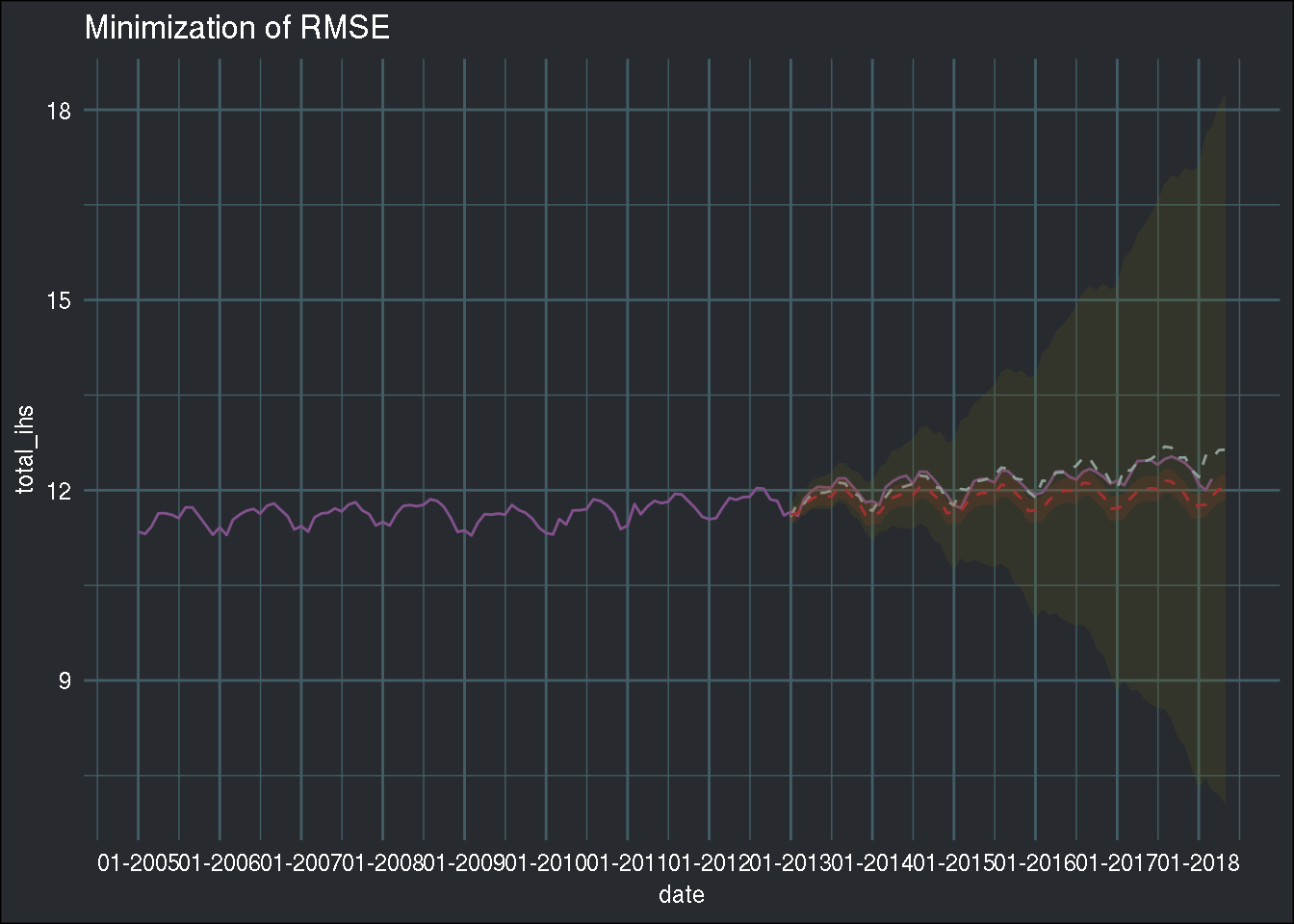
The yellowish line and confidence intervals come from minimizing the genetic algorithm, and the redish from auto.arima(). Interesting; the point estimate is very precise, but the confidence intervals are very wide. Low bias, high variance.
Now, let’s try with another cost function, where I minimize the BIC, similar to the auto.arima() function:
cost_function_bic <- function(param, train_data, validation_data, forecast_periods){
    order <- param[1:3]
    season <- c(param[4:6], 12)
    model <- purrr::possibly(arima, otherwise = NULL)(x = train_data, order = order,
                                                      seasonal = season,
                                                      method = "ML")
    if(is.null(model)){
        return(9999999)
    } else {
        BIC(model)
    }
}
Let’s take a look at the cost at the parameter values returned by auto.arima():
cost_function_bic(c(1, 0, 2, 2, 1, 0),
              train_data = logged_train_data,
              validation_data = logged_validation_data,
              forecast_periods = 65)
## [1] -184.6397Let the genetic algorithm run again:
cl <- makePSOCKcluster(8)
clusterExport(cl, c('logged_train_data', 'logged_validation_data'))

tic <- Sys.time()

auto_arima_bic <- genoud(cost_function_bic,
                     nvars = 6,
                     data.type.int = TRUE,
                     starting.values = c(1, 0, 2, 2, 1, 0), # <- from auto.arima
                     Domains = domains,
                     cluster = cl,
                     train_data = logged_train_data,
                     validation_data = logged_validation_data,
                     forecast_periods = length(logged_validation_data),
                     hard.generation.limit = TRUE)
toc_bic <- Sys.time() - tic
This time, it took 6 minutes, a bit slower than before. Let’s take a look at the solution:
auto_arima_bic## $value
## [1] -201.0656
##
## $par
## [1] 0 1 1 1 0 1
##
## $gradients
## [1] NA NA NA NA NA NA
##
## $generations
## [1] 12
##
## $peakgeneration
## [1] 1
##
## $popsize
## [1] 1000
##
## $operators
## [1] 122 125 125 125 125 126 125 126 0Let’s train the model at these parameters:
best_model_bic <- arima(logged_train_data, order = auto_arima_bic$par[1:3],
                        season = list(order = auto_arima_bic$par[4:6], period = 12),
                        method = "ML")

summary(best_model_bic)
##
## Call:
## arima(x = logged_train_data, order = auto_arima_bic$par[1:3], seasonal = list(order = auto_arima_bic$par[4:6],
## period = 12), method = "ML")
##
## Coefficients:
## ma1 sar1 sma1
## -0.6225 0.9968 -0.832
## s.e. 0.0835 0.0075 0.187
##
## sigma^2 estimated as 0.004145: log likelihood = 109.64, aic = -211.28
##
## Training set error measures:
## ME RMSE MAE MPE MAPE
## Training set 0.003710982 0.06405303 0.04358164 0.02873561 0.3753513
## MASE ACF1
## Training set 0.4553447 -0.03450603And let’s plot the results:
best_model_bic_forecast <- forecast::forecast(best_model_bic, h = 65)

best_model_bic_forecast <- to_tibble(best_model_bic_forecast)
## Joining, by = "date"
## Joining, by = "date"avia_clean_monthly %>%
group_by(date) %>%
summarise(total = sum(passengers)) %>%
mutate(total_ihs = ihs(total)) %>%
ggplot() +
ggtitle("Minimization of BIC") +
geom_line(aes(y = total_ihs, x = date), colour = "#82518c") +
scale_x_date(date_breaks = "1 year", date_labels = "%m-%Y") +
geom_ribbon(data = best_model_bic_forecast, aes(x = date, ymin = lower95, ymax = upper95),
fill = "#5160a0", alpha = 0.2) +
geom_line(data = best_model_bic_forecast, aes(x = date, y = point_estimate),
linetype = 2, colour = "#208480") +
geom_ribbon(data = starting_model_forecast, aes(x = date, ymin = lower95, ymax = upper95),
fill = "#98431e", alpha = 0.2) +
geom_line(data = starting_model_forecast, aes(x = date, y = point_estimate),
linetype = 2, colour = "#a53031") +
theme_blog()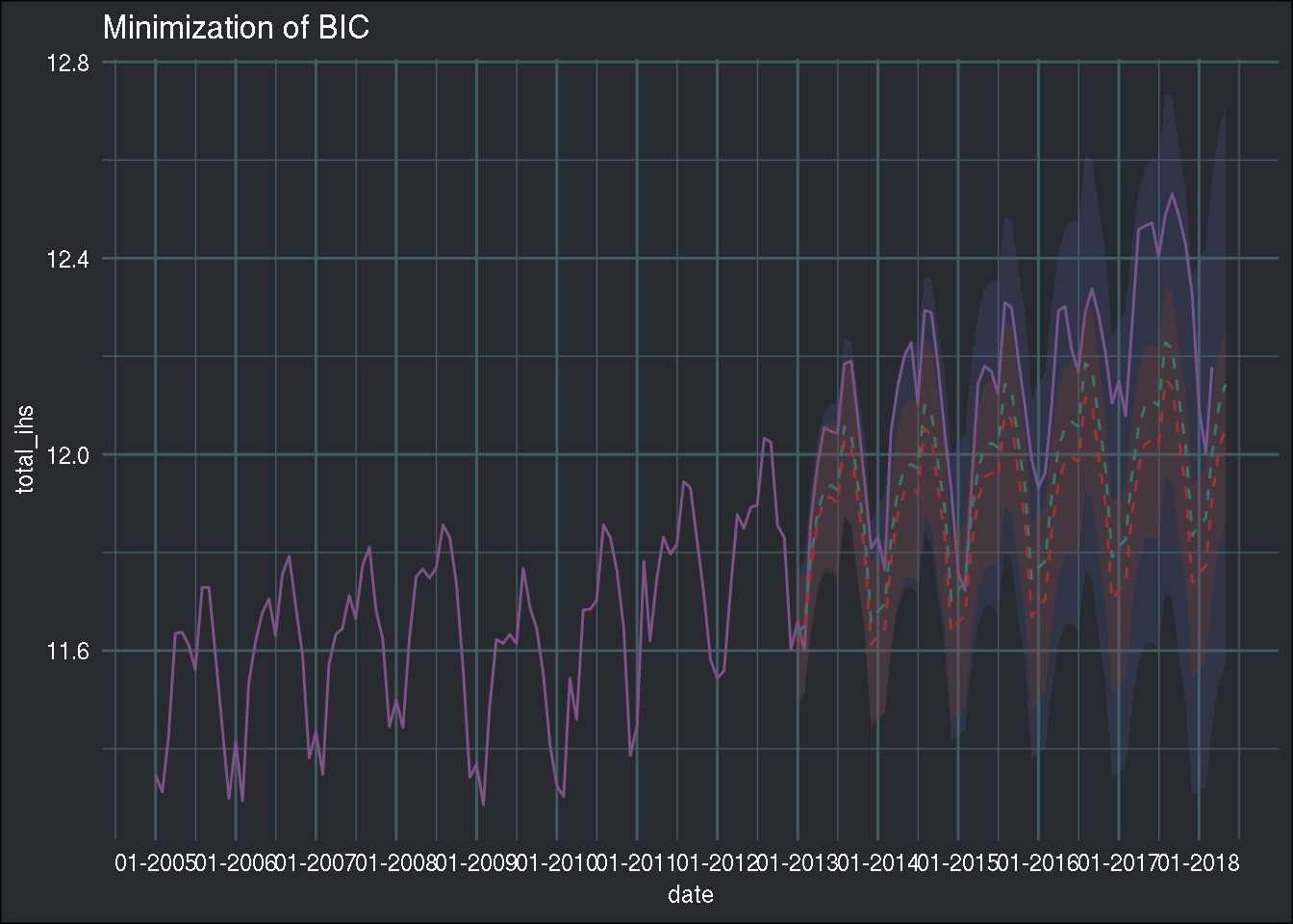
The solutions are very close, both in terms of point estimates and confidence intervals. Bias increased, but variance lowered… This gives me an idea! What if I minimize the RMSE, while keeping the number of parameters low, as a kind of regularization? This is somewhat what minimising BIC does, but let’s try to do it a more “naive” approach:
cost_function_rmse_low_k <- function(param, train_data, validation_data, forecast_periods, max.order){
    order <- param[1:3]
    season <- c(param[4:6], 12)
    if(param[1] + param[3] + param[4] + param[6] > max.order){
        return(9999999)
    } else {
        model <- purrr::possibly(arima, otherwise = NULL)(x = train_data,
                                                          order = order,
                                                          seasonal = season,
                                                          method = "ML")
    }
    if(is.null(model)){
        return(9999999)
    } else {
        forecast_model <- forecast::forecast(model, h = forecast_periods)
        point_forecast <- forecast_model$mean
        sqrt(mean(point_forecast - validation_data) ** 2)
    }
}
This is also similar to what auto.arima() does; by default, the max.order argument in auto.arima() is set to 5, and is the sum of p + q + P + Q. So I’ll try something similar.
Let’s take a look at the cost at the parameter values returned by auto.arima():
cost_function_rmse_low_k(c(1, 0, 2, 2, 1, 0),
              train_data = logged_train_data,
              validation_data = logged_validation_data,
              forecast_periods = 65,
              max.order = 5)
## [1] 0.1731473Let’s see what will happen:
cl <- makePSOCKcluster(8)
clusterExport(cl, c('logged_train_data', 'logged_validation_data'))

tic <- Sys.time()

auto_arima_rmse_low_k <- genoud(cost_function_rmse_low_k,
                         nvars = 6,
                         data.type.int = TRUE,
                         starting.values = c(1, 0, 2, 2, 1, 0), # <- from auto.arima
                         max.order = 5,
                         Domains = domains,
                         cluster = cl,
                         train_data = logged_train_data,
                         validation_data = logged_validation_data,
                         forecast_periods = length(logged_validation_data),
                         hard.generation.limit = TRUE)
toc_rmse_low_k <- Sys.time() - tic
It took 1 minute to train this one, quite fast! Let’s take a look:
auto_arima_rmse_low_k## $value
## [1] 0.002503478
##
## $par
## [1] 1 2 0 3 1 0
##
## $gradients
## [1] NA NA NA NA NA NA
##
## $generations
## [1] 11
##
## $peakgeneration
## [1] 1
##
## $popsize
## [1] 1000
##
## $operators
## [1] 122 125 125 125 125 126 125 126 0And let’s plot it:
best_model_rmse_low_k <- arima(logged_train_data, order = auto_arima_rmse_low_k$par[1:3],
                               season = list(order = auto_arima_rmse_low_k$par[4:6], period = 12),
                               method = "ML")

summary(best_model_rmse_low_k)
##
## Call:
## arima(x = logged_train_data, order = auto_arima_rmse_low_k$par[1:3], seasonal = list(order = auto_arima_rmse_low_k$par[4:6],
## period = 12), method = "ML")
##
## Coefficients:
## ar1 sar1 sar2 sar3
## -0.6468 -0.7478 -0.5263 -0.1143
## s.e. 0.0846 0.1171 0.1473 0.1446
##
## sigma^2 estimated as 0.01186: log likelihood = 57.88, aic = -105.76
##
## Training set error measures:
## ME RMSE MAE MPE MAPE
## Training set 0.0005953302 0.1006917 0.06165919 0.003720452 0.5291736
## MASE ACF1
## Training set 0.6442205 -0.3706693best_model_rmse_low_k_forecast <- forecast::forecast(best_model_rmse_low_k, h = 65)
best_model_rmse_low_k_forecast <- to_tibble(best_model_rmse_low_k_forecast)## Joining, by = "date"
## Joining, by = "date"avia_clean_monthly %>%
group_by(date) %>%
summarise(total = sum(passengers)) %>%
mutate(total_ihs = ihs(total)) %>%
ggplot() +
ggtitle("Minimization of RMSE + low k") +
geom_line(aes(y = total_ihs, x = date), colour = "#82518c") +
scale_x_date(date_breaks = "1 year", date_labels = "%m-%Y") +
geom_ribbon(data = best_model_rmse_low_k_forecast, aes(x = date, ymin = lower95, ymax = upper95),
fill = "#5160a0", alpha = 0.2) +
geom_line(data = best_model_rmse_low_k_forecast, aes(x = date, y = point_estimate),
linetype = 2, colour = "#208480") +
geom_ribbon(data = starting_model_forecast, aes(x = date, ymin = lower95, ymax = upper95),
fill = "#98431e", alpha = 0.2) +
geom_line(data = starting_model_forecast, aes(x = date, y = point_estimate),
linetype = 2, colour = "#a53031") +
theme_blog()
Looks like this was not the right strategy. There might be a better cost function than what I have tried, but looks like minimizing the BIC is the way to go.