R or Python? Why not both? Using Anaconda Python within R with {reticulate}

This short blog post illustrates how easy it is to use R and Python in the same R Notebook thanks to the {reticulate} package. For this to work, you might need to upgrade RStudio to the current preview version. Let’s start by importing {reticulate}:
library(reticulate)
{reticulate} is an RStudio package that provides “a comprehensive set of tools for interoperability between Python and R”. With it, it is possible to call Python and use Python libraries within an R session, or define Python chunks in R markdown. I think that using R Notebooks is the best way to work with Python and R; when you want to use Python, you simply use a Python chunk:
```{python}
your python code here
```
There’s even autocompletion for Python object methods:
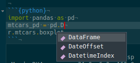
Fantastic!
However, if you wish to use Python interactively within your R session, you must start the Python REPL with the repl_python() function, which starts a Python REPL. You can then do whatever you want, even access objects from your R session, and then when you exit the REPL, any object you created in Python remains accessible in R. I think that using Python this way is a bit more involved and would advise using R Notebooks if you need to use both languages.
I installed the Anaconda Python distribution to have Python on my system. To use it with {reticulate} I must first use the use_python() function that allows me to set which version of Python I want to use:
# This is an R chunk
use_python("~/miniconda3/bin/python")
I can now load a dataset, still using R:
# This is an R chunk
data(mtcars)
head(mtcars)
## mpg cyl disp hp drat wt qsec vs am gear carb
## Mazda RX4 21.0 6 160 110 3.90 2.620 16.46 0 1 4 4
## Mazda RX4 Wag 21.0 6 160 110 3.90 2.875 17.02 0 1 4 4
## Datsun 710 22.8 4 108 93 3.85 2.320 18.61 1 1 4 1
## Hornet 4 Drive 21.4 6 258 110 3.08 3.215 19.44 1 0 3 1
## Hornet Sportabout 18.7 8 360 175 3.15 3.440 17.02 0 0 3 2
## Valiant 18.1 6 225 105 2.76 3.460 20.22 1 0 3 1
and now, to access the mtcars data frame, I simply use the r object:
# This is a Python chunk
print(r.mtcars.describe())
## mpg cyl disp ... am gear carb
## count 32.000000 32.000000 32.000000 ... 32.000000 32.000000 32.0000
## mean 20.090625 6.187500 230.721875 ... 0.406250 3.687500 2.8125
## std 6.026948 1.785922 123.938694 ... 0.498991 0.737804 1.6152
## min 10.400000 4.000000 71.100000 ... 0.000000 3.000000 1.0000
## 25% 15.425000 4.000000 120.825000 ... 0.000000 3.000000 2.0000
## 50% 19.200000 6.000000 196.300000 ... 0.000000 4.000000 2.0000
## 75% 22.800000 8.000000 326.000000 ... 1.000000 4.000000 4.0000
## max 33.900000 8.000000 472.000000 ... 1.000000 5.000000 8.0000
##
## [8 rows x 11 columns]
.describe() is a Python Pandas DataFrame method to get summary statistics of our data. This means that mtcars was automatically converted from a tibble object to a Pandas DataFrame! Let’s check its type:
# This is a Python chunk
print(type(r.mtcars))
## <class 'pandas.core.frame.DataFrame'>Let’s save the summary statistics in a variable:
# This is a Python chunk
summary_mtcars = r.mtcars.describe()
Let’s access this from R, by using the py object:
# This is an R chunk
class(py$summary_mtcars)
## [1] "data.frame"Let’s try something more complex. Let’s first fit a linear model in Python, and see how R sees it:
# This is a Python chunk
import numpy as np
import statsmodels.api as sm
import statsmodels.formula.api as smf
model = smf.ols('mpg ~ hp', data = r.mtcars).fit()
print(model.summary())
## OLS Regression Results
## ==============================================================================
## Dep. Variable: mpg R-squared: 0.602
## Model: OLS Adj. R-squared: 0.589
## Method: Least Squares F-statistic: 45.46
## Date: Sun, 10 Feb 2019 Prob (F-statistic): 1.79e-07
## Time: 00:25:51 Log-Likelihood: -87.619
## No. Observations: 32 AIC: 179.2
## Df Residuals: 30 BIC: 182.2
## Df Model: 1
## Covariance Type: nonrobust
## ==============================================================================
## coef std err t P>|t| [0.025 0.975]
## ------------------------------------------------------------------------------
## Intercept 30.0989 1.634 18.421 0.000 26.762 33.436
## hp -0.0682 0.010 -6.742 0.000 -0.089 -0.048
## ==============================================================================
## Omnibus: 3.692 Durbin-Watson: 1.134
## Prob(Omnibus): 0.158 Jarque-Bera (JB): 2.984
## Skew: 0.747 Prob(JB): 0.225
## Kurtosis: 2.935 Cond. No. 386.
## ==============================================================================
##
## Warnings:
## [1] Standard Errors assume that the covariance matrix of the errors is correctly specified.Just for fun, I ran the linear regression with the Scikit-learn library too:
# This is a Python chunk
import numpy as np
from sklearn.linear_model import LinearRegression
regressor = LinearRegression()
x = r.mtcars[["hp"]]
y = r.mtcars[["mpg"]]
model_scikit = regressor.fit(x, y)
print(model_scikit.intercept_)
## [30.09886054]print(model_scikit.coef_)## [[-0.06822828]]
Let’s access the model variable in R and see what type of object it is in R:
# This is an R chunk
model_r <- py$model
class(model_r)
## [1] "statsmodels.regression.linear_model.RegressionResultsWrapper"
## [2] "statsmodels.base.wrapper.ResultsWrapper"
## [3] "python.builtin.object"So because this is a custom Python object, it does not get converted into the equivalent R object. This is described here. However, you can still use Python methods from within an R chunk!
# This is an R chunk
model_r$aic
## [1] 179.2386model_r$params## Intercept hp
## 30.09886054 -0.06822828
I must say that I am very impressed with the {reticulate} package. I think that even if you are primarily a Python user, this is still very interesting to know in case you need a specific function from an R package. Just write all your script inside a Python Markdown chunk and then use the R function you need from an R chunk! Of course there is also a way to use R from Python, a Python library called rpy2 but I am not very familiar with it. From what I read, it seems to be also quite simple to use.